How to Use Functions in Google Sheets

Last Updated: November 8, 2021

This wikiHow teaches you how to use basic functions in Google Sheets. A function is used in a formula to make a calculation based on cell values, such as finding the total of a group of cells.

Steps

1
Learn the syntax of a formula. “Syntax” refers to the correct order in which you must type the formula. If the syntax is incorrect, you’ll get an error instead of a proper result. The syntax for a formula is =FUNCTION_NAME(ARGUMENT).
- For example, let’s say we want to write a formula that finds the sum of all values from cells A1 through A10. The formula would look like this: =SUM(A1:A10).
  - =SUM is the function. Sheets has built-in functions you can add to formulas. All functions begin with an equal sign =.
  - (A1:A10) is the argument (the cells the function will use).
- This example only has one argument. If you’re doing a more complex function that requires more than one range, each range will be separated by a comma.
  - An example of a multi-argument formula: To find the sum cells A1 to A10, B3 to B5, and C1, the formula would be =SUM(A1:A10,B3:B5,C1).
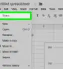
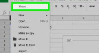
2
Open a spreadsheet in Google Sheets. Now you’ll create a new formula that uses a basic function. If you haven’t already done so, sign into your Google Drive (https://drive.google.com), then click the sheet you want to edit.
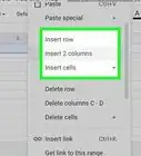
- If you’re creating a new sheet, type some numerical values into the cells in the first few columns so you have something to work with.
3
Click an empty cell. This is where you will type the formula. When the function runs against the arguments, the results will appear in this cell.
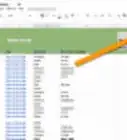
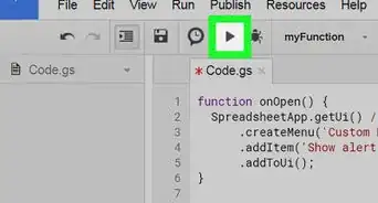
4
Click the function button. It’s the last icon in the toolbar at the top of the screen. It looks like a sideways “M” or a more angular “E.” A menu of functions will expand.
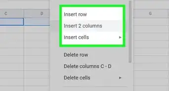
5
Click the function you want to use. Since we’re just getting started, select SUM. This inserts =SUM() into the selected cell. The mouse cursor is positioned between the two parentheses, ready for you to enter or select cells.
- If you know which function you need, click More functions… to view other options, then select the function from the list.
- Some basic functions besides SUM are AVERAGE (find the average value in a range), MAX (find the highest value), and MIN (find the lowest value).
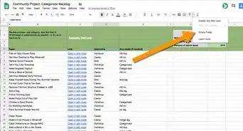
6
Add the argument. Let’s say we want to find the sum of all values in the first 6 rows of columns A, B, and C. There are two ways to enter this range:
- Use the mouse to select/highlight columns A, B, and C down to the 6th row. This automatically inserts the range A1:C6 between the parentheses.
- Type the range manually. Enter the first cell (A1), a colon (:), and then the last cell in the range (C6). The argument would look like this: A1:C6
7
Press ↵ Enter or ⏎ Return. This runs the formula. The sum of the selected cells will appear in place of the formula you entered.
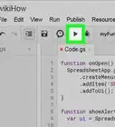
8
Enter a formula manually. While it’s quick and easy to click the function button in the toolbar, you can manually type formulas if you know the name of the function. Just remember the syntax: {kbd|=FUNCTION_NAME(ARGUMENT)}}.
- Example: Type =MIN(A1:C6) into a cell and press ↵ Enter or ⏎ Return.
- The smallest value of the range will now appear in the cell in which you typed the formula.