How to Filter on Google Sheets on PC or Mac

Co-authored by wikiHow Staff

Last Updated: May 15, 2018

This wikiHow teaches you how to filter and hide cells by value or condition in a Google Sheets spreadsheet, using a computer.

Steps

1
Open Google Sheets in an internet browser. Type sheets.google.com into the address bar, and hit ↵ Enter or ⏎ Return on your keyboard.
2
Click the spreadsheet you want to edit. Find the spreadsheet you want to filter on your list of saved sheets, and open it.
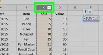
3
Select the range of cells you want to filter. Click the first cell in the data range, and drag your mouse to select its adjacent cells.
4
Click the Filter icon on the toolbar. This icon looks like a funnel cone next to the function icon at the top of your spreadsheet. It will bold the first cell in your selected data range.
5
Click the three horizontal lines icon in the first cell of your cell range. This will open a pop-up menu.
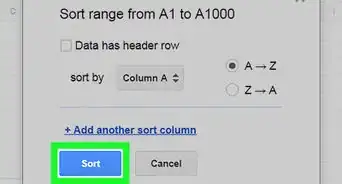
6
Select a filter to apply to the selected cells. You can find a list of available conditional filters in the Filter by condition section, or manually enter a numeric value in the Filter by values section.
- If you select Filter by condition, click the drop-down menu and select a filter to apply.
- If you select Filter by values, enter the values you want to filter into the text box.
7
Click the blue OK button. This will filter the selected data range, and hide the filtered cells from your spreadsheet.

You Might Also Like

About This Article

Co-authored by:

wikiHow Staff Writer

This article was co-authored by wikiHow Staff. Our trained team of editors and researchers validate articles for accuracy and comprehensiveness. wikiHow's Content Management Team carefully monitors the work from our editorial staff to ensure that each article is backed by trusted research and meets our high quality standards. This article has been viewed 2,451 times.

How helpful is this?

Co-authors: 2

Updated: May 15, 2018

Views: 2,451

Categories: Google Applications

Article SummaryX

1. Open Google Sheets.
2. Click a spreadsheet.
3. Select a cell range.
4. Click the Filter icon on the toolbar.
5. Click the three horizontal lines icon in your first cell.
6. Select a filter type.
7. Click OK.

Did this summary help you?